In this blog post I will introduce a GxExM prediction problem, dive into the data, and explain the results.
The task in this problem is to predict a double extrapolation effect, in this case, our training data is missing to key components; a unique location * water combination, and a new planting density. This comes with many challenges which will be highlighted below.
For our training data we are given replicated trial data for 1500 inbred lines genotyped with: 1) ~500 SNP markers 2) 2 replicates for Yield values for the following locations and water levels: Emerald Dry, Dalby Dry, and Dalby Wet grown at 25 and 50 planting density 3) 3 traits or ‘historical covariates’; these are the average values of the genotypes grown in 3 distinct environments (outside of our training/test data) for tillering, maturity, and leaf size.
Again, our goal is to use this training data to predict yields for Emerald Wet at 75 planting density. This exclusion of Emerald * Wet and planting density 75 means we are trying to doubly extract the effect of location * wet and increasing the planting density. This is a very difficult problem which limits our modeling approach.
First we will do an exploratory data analysis of the training dataset. We can calculate the broad-sense heritability of yield (our target to predict) thanks to having 2 replicates of each genotype for each location * wet * planting density.
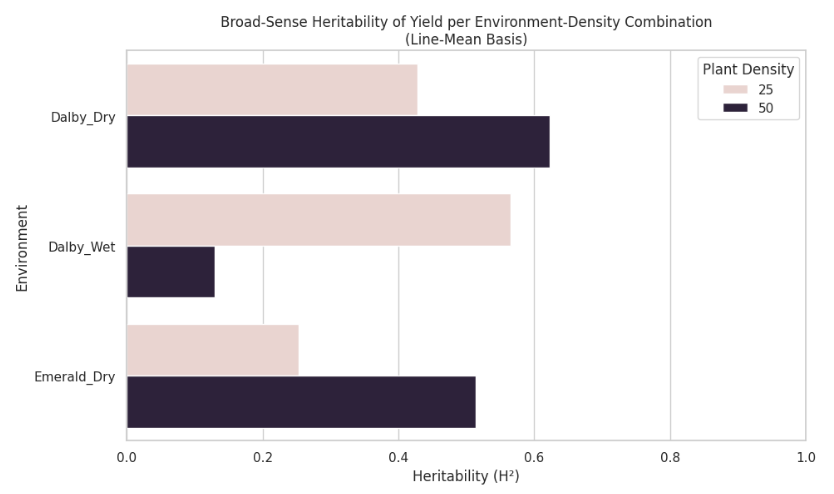
The major points to note are that the heritability of yield vary drastically, suggesting that environment interactions play a strong role in the yield. Notably, in Dalby Wet at 50 planting density, heritability is the lowest. This is foreshadowing for our model; telling us that the environmental features in the model will have a greater effect than the SNP marker data.
Next we will look at the correlations between the yields of each trial location, planting density, dry versus wet condition with the 3 historical covariates and the PCA’s of the marker data.
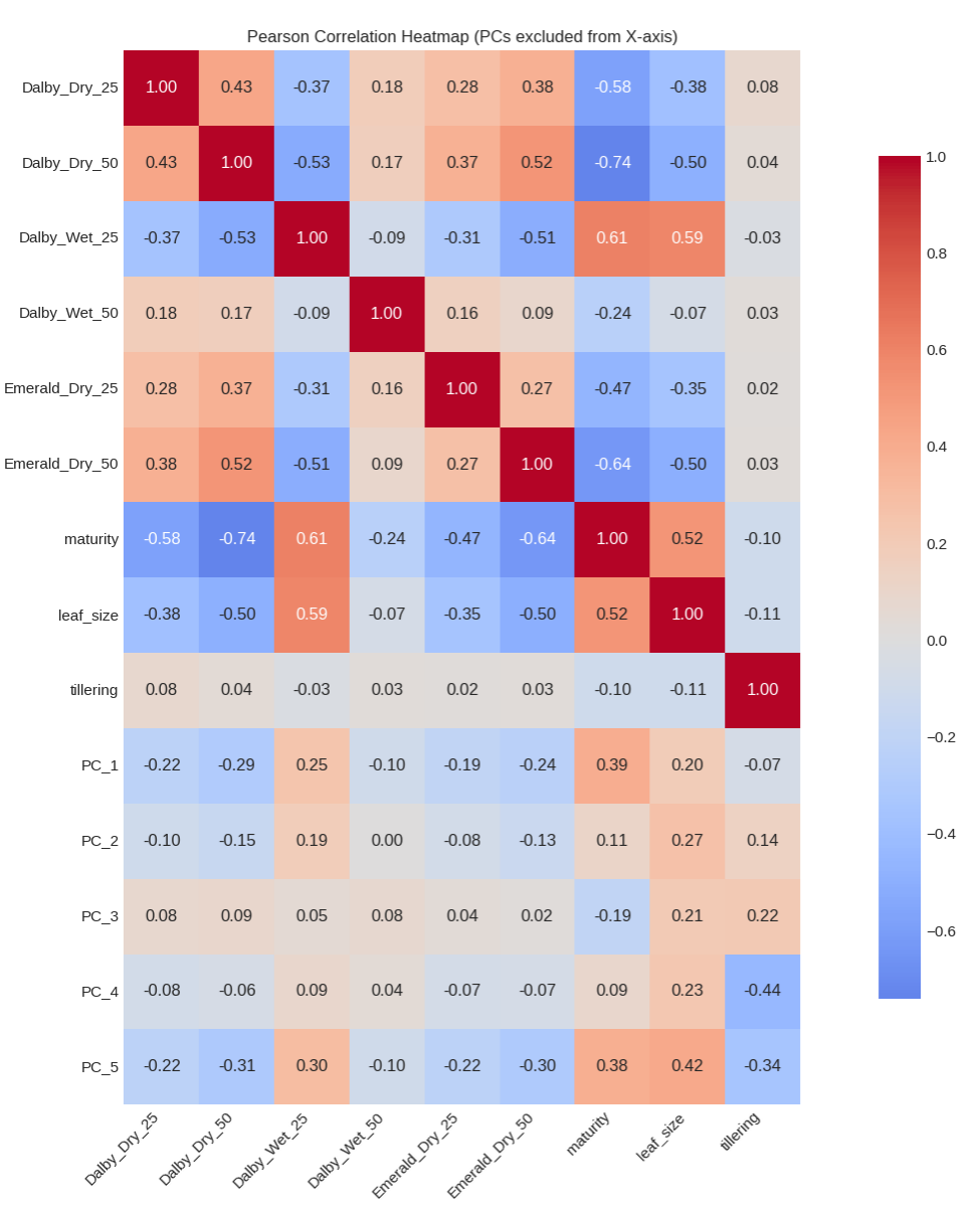
This is is a dense summary of the training dataset. Notable features include: 1) The correlation between Dalby 25 Wet and other environments is, uniquely, negative. This means that the yield scores completely switch; the top performers in the other environments are not the same in Dalby 25 Wet. This is likely because at low density, and high resources, different genotypes perform better with less stress versus the genotypes that yield higher under competition and fewer resources 2) Dalby 25 Wet and Dalby 50 Wet have a negative correlation; Despite being in the same location and water condition, there is a significant difference in performance similar to the previous point. Maturity is a strong indicator of this; it actually sign flips indicating that early maturity backfires in the low stress environment in Dalby 25 Wet whereas in Dalby 50 wet, maturing early allows the yield to stay high in the presence of different stresses. 3) The high correlations between the historical covariates suggest that these are extremely valuable traits for our models
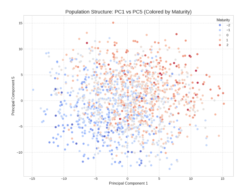
Now onto the PC’s of the genotype data. To compress the 500 markers into fewer features PCA was used to identify principal components to act as stand-ins for the raw marker data. Interestingly, many of the PCs share similar correlation profiles. These PCs represent linkage disequilibrium and population effects from previous rounds of selection. The training data is not random cultivars, but likely originated from aggregating sub populations which were selected for traits like maturity or leaf size. Indeed, some of the PCs have very strong correlations with maturity, as we can see in this colored PCA plot, suggesting that the PCs and historical covariates share a lot of the same information.
Modeling
Due to the experimental design, linear models are the best fit. While conventional machine learning models may perform better with predictions under similar distributions (within the training data set) our prediction task is double extrapolation. As a result, we must use linear models which capture correlation between our features.
Linear models require feature engineering, so we created a suite of models with explicit interactions between our features of interest, like the wet condition, plant density, location, and the historical covariates.
An Elastic Net model was used for this; it’s a linear model which can be tuned to act as a ridge regression (shrinks every feature closer to 0 with penalties) versus LASSO which can capture co-linearity between multiple features and group their features together to account for collinearity.
Cross Validation
This is difficult to do for this particular task. Traditionally, we would leave a single environment out and train on the rest of the environments. However, since we are doing double extrapolation, each of the cross validation tasks will be missing a critical feature seen in only the left-out environment. Instead we picked the the most relevant environment * condition combinations for the prediction task of Emerald 75 Wet. Additionally we included a cross validation fold for prediciting Dalby2Emerald and planting density 25 to 50. Given the experimental design, this is the best we can do.
Notably, our previous exploratory data analysis is reaffirmed in the results of the suite of models; no model performed better than the baseline model (a simple model with the basic features of environment/planting density and historical covariates) for Dalby 50 Wet, likely due to the low heritability mentioned earlier.
M4 is the best overall, although not the best in every cross validation fold. Including the wet x density feature allowed it to disentangle the interaction effects and capture the Dalby2Emerald fold, this is because the only Emerald training data was Dry. Without this feature, the linear model is forced to use the correlations from the wet environments explicitly in its predictions.
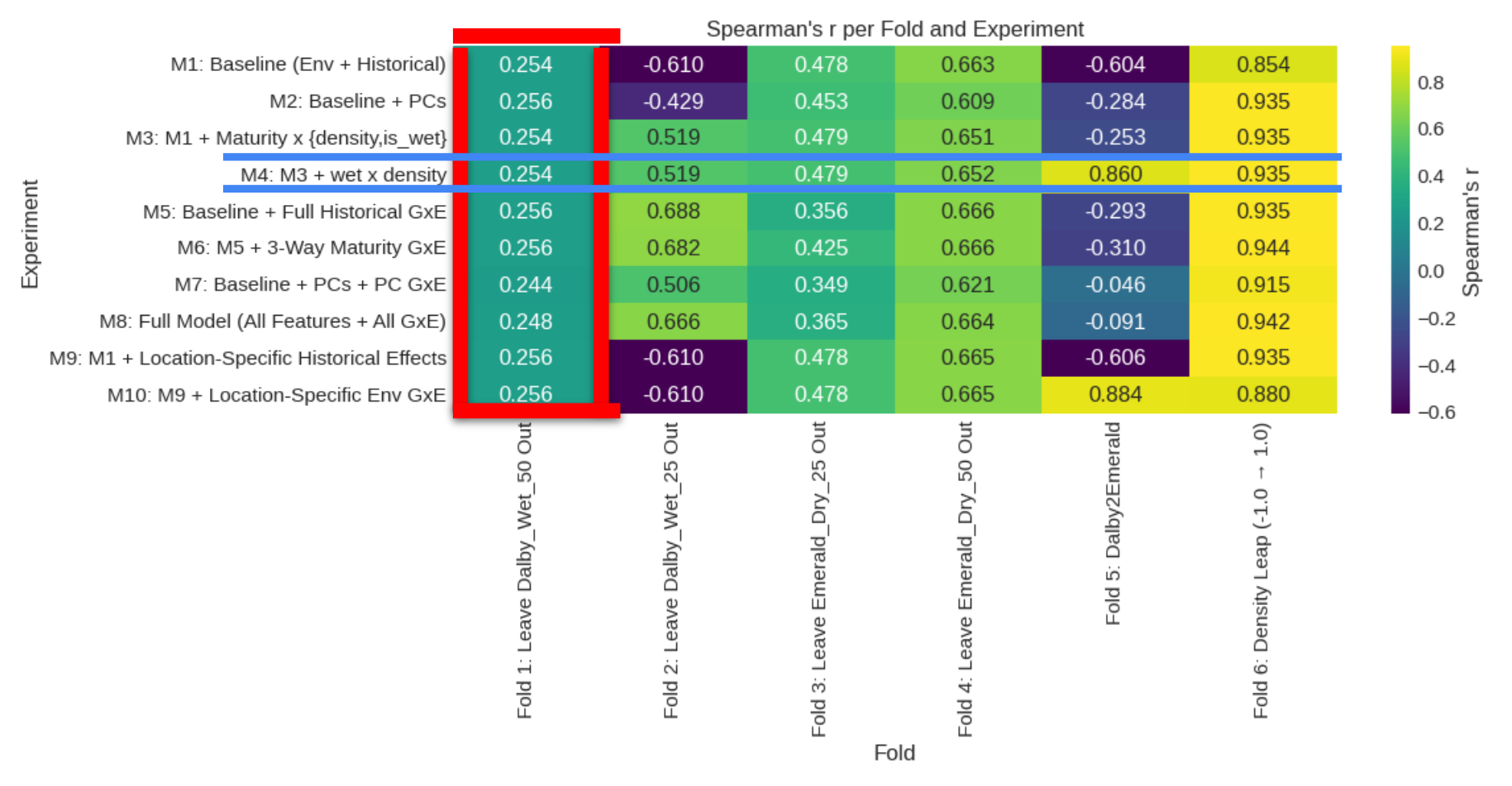
Despite models M5-M10 including many more features, M4 is relatively simple and effective. We will use it as our final model to predict the Emerald 75 Wet test dataset.
Results
Here we can see that the simple model was able to achieve a high correlation with predictions versus truth, by leveraging the entire training dataset. The scales of the predictions (x and y axis) appear far off, however, this is due to some preprocessing (calculating BLUEs) and the fact that the wet environments have the highest overall yields and our linear model was trained largely on dry environments.
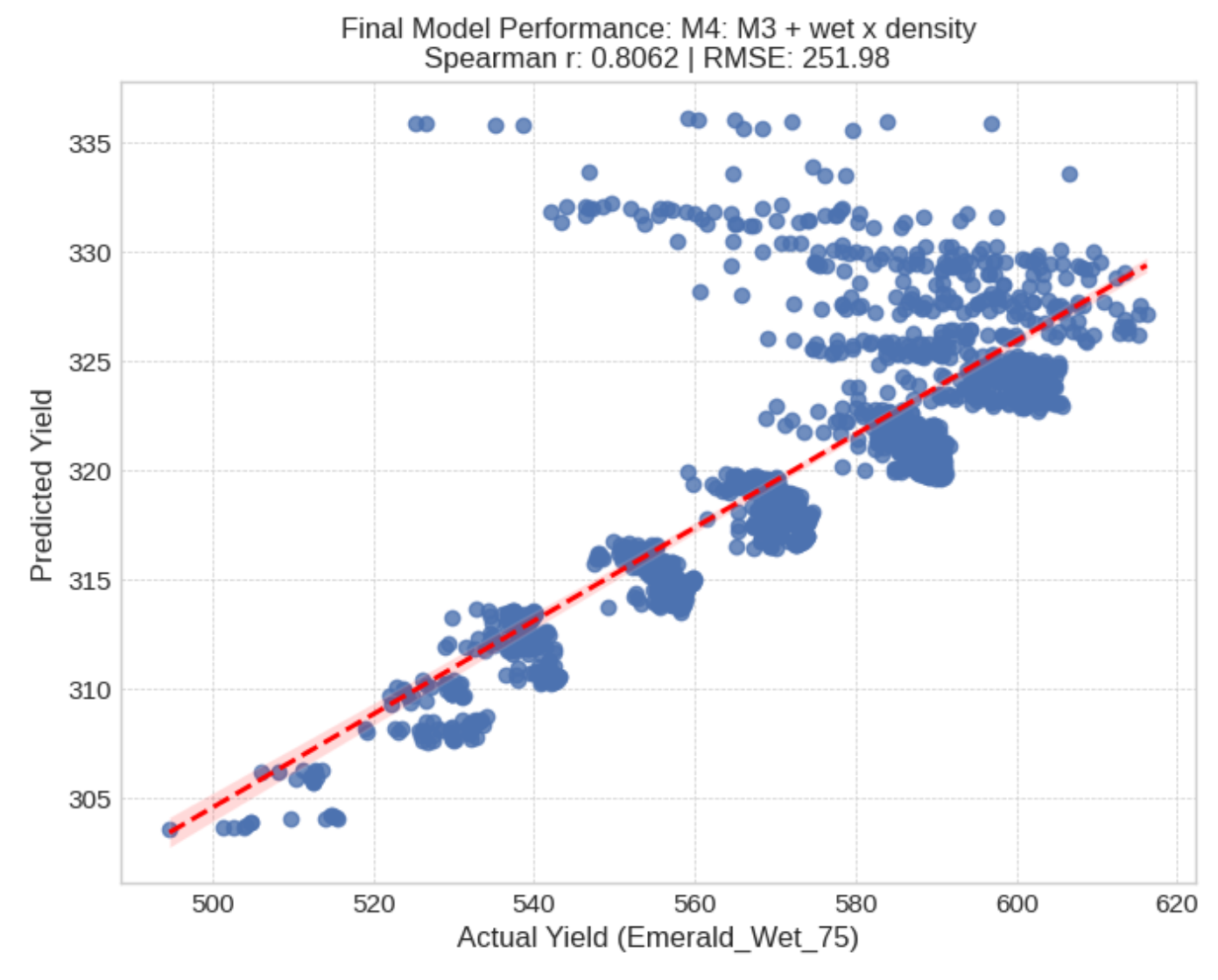
The clusters are due to one of the input features; tillering, which was effectively a categorical variable. We also notice a cluster on the top of genotypes which did not follow the same linear pattern as the rest of the data points. This is likely due to non-additive genetic interactions in these particular cultivars. Some cultivars are ‘specialists’ possessing more genes that have interactions with the environment which is not captured by our simple linear model. Conversely, some cultivars are more stable across the different conditions lacking these interactions.
Overall, this prediction tasks highlights the critical link between experimental design and model selection. If we weren’t doing double extraction we could have leveraged non-linear models like XGBoost, random forest, or neural networks. However these suffer with unseen features, for instance tree-based models would be forced to ‘clamp’ down at nodes where the data is split by plant density. Since they have not seen 75 density in the training data they would be forced to traverse down 50 density, losing the interaction completely.
This constraint also prevents us from using non-linear models and linear models in 2 part prediction models. For example, using the non-linear models to predict the errors from the linear model, and correcting it. Residual learning would be a powerful approach otherwise.